From the Not Just Numbers blog:

Before getting into today’s post I want to point you to an excellent free Webinar being offered (for a limited time) by Mynda Treacy, entitled “Creating Excel Dashboards“. Mynda is a real expert on Excel Dashboards and her training materials are always excellent. You can register for the webinar here.

I realised the other day that I had never covered one of my most used functions on this blog – SUMIFS. I have covered its predecessor, SUMIF, as SUMIFS has only been available since Excel 2007.

Although SUMIF is still available in later versions of Excel for compatibility purposes, it is essentially redundant, as SUMIFS does the same thing, plus a lot more.

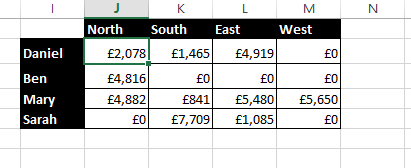
Let us look at an example of some sales data (see left).

Say we want to know how much Mary’s sales were, or how much Sarah sold in the East Region, or even how much Ben sold in the North region in the month of January.

SUMIFS can do all of these.

The syntax for SUMIFS is as follows:

=SUMIFS(SumRange,CriteriaRange1,Criteria1,[CriteriaRange2],[Criteria2]…..)

You can have as many pairs of CriteriaRange and Criteria as you need. The function works as follows:

SUM SumRange where CriteriaRange1 = Criteria1 and CriteriaRange2 = Criteria2 etc. for however many criteria you have.

For all of the examples above the SumRange will be D2:D21, as this is the range we want to sum, subject to our criteria. We will look at how we construct the rest of the formula for each of our examples above.

How much did Mary sell?
Here we only have one criteria:

CriteriaRange1 = C2:C21
Criteria1 = “Mary”

=SUMIFS(D2:D21,C2:C21,”Mary”)

returns £16,853.


How much did Sarah sell in the East Region?
This time we have two criteria:

CriteriaRange1 = C2:C21
Criteria1 = “Sarah”

CriteriaRange2 = B2:B21
Criteria2 = “East”

=SUMIFS(D2:D21,C2:C21,”Sarah”,B2:B21,”East”)


returns £1,085.

How much did Ben sell in the North Region in the month of January?
This time we actually have four criteria:

CriteriaRange1 = C2:C21
Criteria1 = “Ben”

CriteriaRange2 = B2:B21
Criteria2 = “North”

CriteriaRange3 = A2:A21
Criteria3 = “>=”&DATE(2016,1,1)

CriteriaRange4 = A2:A21
Criteria4 = “<=”&DATE(2016,1,31)

There are two elements to these last two criteria that need further explanation.

The first is that if our criteria is anything other than equals, we need to include the criteria in inverted commas, for example “>23”, or “<=15”, to make it a string. If rather than 23, we wished to refer to a cell (say G5) we can use the ampersand (&) to join two strings together, e.g. “>”&G5.

The second is that if we wish to refer to a date directly, we need to refer its sequential number which we can calculate using the DATE function. The three arguments for the DATE function are Year, Month and Day, so to get the date sequence number for 1st January 2016, we can use DATE(2016,1,1). Note that if we entered 1/1/2016 in cell G5, we could just use “>=”&G5 for Criteria3, as the cell value when you enter a date, is its date sequence value.

Our function is therefore:

If you enjoyed this post, go to the top of the blog, where you can subscribe for regular updates and get two freebies “The 5 Excel features that you NEED to know” and “30 Chants for Better Charts”.

From the Not Just Numbers blog:

Let me start with an apology. My current workload has meant that my posts have been a lot less frequent in recent weeks. This may continue for a while, but I will still be aiming to post at least once a month during this busy spell.

In this post I want to show you how to do something I have shown before using OFFSET, but this time using the more efficient INDEX.

Let’s look at the example of a 12 month budget spreadsheet with the monthly sales figures in cells B9 to M9 (month 1 in B9, Month 2 in C9, etc.). And let’s say that the current month number is entered in cell B6.

Using OFFSET we could return the current month’s sales using:

=OFFSET($B9,0,$B$6-1)

and the cumulative sales using:

=SUM(OFFSET($B9,0,0,1,$B$6))

See this earlier post, if you don’t understand why.

The problem with OFFSET though, is that it is what is known as a “volatile” function. This means that it always has to be recalculated when any cell in the spreadsheet changes – as it does not specify a range that it is dependent on, therefore does not know whether a change might affect its result.

INDEX however looks at a defined range, making it significantly more efficient, and in its simplest form can be used to replace both of these examples of OFFSET.

For a range the width of a single cell (as in our example), INDEX only needs two arguments to return the current month’s sales:

=INDEX($B9:$M9,$B$6)

This returns the value of the cell in position B6 in the range B9:M9.

If $B$6 is 3, this will return the value in cell D9, being the third cell in the range B9:M9.

To do the cumulative calculation, we can use the same INDEX function to return the end of  a SUM range, while fixing the start:

=SUM($B9:INDEX($B9:$M9,$B$6))

Again, if B6 contains 3, then this returns the sum of the range B9:D9.

In both cases, these will only recalculate if a cell in the range B9:M9 is edited. In a complex spreadsheet with many calculations, this can make a huge difference to calculation times.

If you enjoyed this post, go to the top of the blog, where you can subscribe for regular updates and get two freebies “The 5 Excel features that you NEED to know” and “30 Chants for Better Charts”.

From the Not Just Numbers blog:

One of the challenges that many Excel users face, is ensuring that the printed version of a spreadsheet looks as good as it did on the screen.

There are a few simple things that you need to know to help to organise what actually gets printed and how it is spread across pages.

I will cover the first of these today, and revisit some of the others in future posts.

Today we will look at how to determine how much of the sheet is actually printed.

Left to its own devices, Excel will print all of the used area on the sheet, Specifically, it will print the whole area from cell A1 to the rightmost column and the last row that are not empty.

This may not be what is required, and it is easy to change. Simply highlight the area that you do want to print, then go to the Page Layout ribbon, click the Print Area icon, and select Set Print Area.

You can even select multiple ranges (holding down the Control key, while you select the subsequent ranges) which Excel will print on different pages.

For example, you may have a Profit & Loss and Balance Sheet alongside each other on one worksheet. Just highlight the area of the Profit and Loss (say A1:H100) and then hold down the Control key while selecting the Balance Sheet range (say J1:P80) and Set Print Area as described above.

Once a Print Area has been set in this way, you can see (and edit it) using the Name Manager on the Formulas ribbon. You will see all of the Print Areas in the workbook listed there and (scope to their particular worksheet). You can then edit these ranges like any other.

You can even make them a dynamic range using functions like OFFSET and INDEX, so that the area that gets printed is determined by values in the workbook.

A particularly useful technique is to combine this ability to set a dynamic Print Area with a formula to determine the last row of data. I explained a formula to do this in this earlier post.

Let’s say we put this formula in a cell that we name LastRow.

If we want the print area to be columns A to J but the height of the print area to flex to the amount of rows occupied, we can enter the following as the Print Area (in the Names Manager):

=OFFSET($A$1,0,0,LastRow,10)

This will print a range starting at A1, with a height of LastRow, and a width of 10 (A to J is 10 columns).

If you enjoyed this post, go to the top of the blog, where you can subscribe for regular updates and get two freebies “The 5 Excel features that you NEED to know” and “30 Chants for Better Charts”.

From the Not Just Numbers blog:

Before I begin, I would like to wish a Happy New Year to all of my readers and subscribers – as this is my first post of 2016.

I am starting the year in humble mode, as I have had something very simple pointed out to me that I can’t believe I had never spotted, despite it being right under my nose!

In my last post of 2015, I showed you some code to swap one cell colour for another throughout a worksheet. I then received a comment from a reader that I only know as Jim, pointing out that Excel already has a very simple way of doing this!

It can in fact be done using Find and Replace.

This amazed me because I use Find and Replace all of the time and didn’t know you could do this!

It is simple as this:

1. Highlight the range which you want to apply the changes to
2. Click Find and Select (the binoculars icon) on the Home Ribbon and choose Replace from the dropdown menu
3. Don’t enter anything in the Find or Replace boxes, but click the Format button next to the Find box and on the Fill Tab, select the colour that you wish to change
4. Click the Format box next to the Replace box and on the Fill Tab, select the new colour that you wish to swap for the colour you selected above
5. Click Replace All

If you enjoyed this post, go to the top of the blog, where you can subscribe for regular updates and get two freebies “The 5 Excel features that you NEED to know” and “30 Chants for Better Charts”.

From the Not Just Numbers blog:

First of all I would like to wish all of my readers and subscribers, a very Merry Christmas and a Happy 2016.

I know we all work hard, and I hope, like me, you all get a chance to spend some time with those you love in the coming days, whether Christmas is a festival you celebrate or not.

One hassle I sometimes have when building spreadsheets for others is changing colours.

The spreadsheet may work perfectly, but the end user might not like the colours I have chosen. This isn’t too much of a problem if we are talking about large blocks of colour, but it can be a time-taking process, if I have used yellow to denote input cells throughout the whole worksheet, and the client wants orange, for example!

When this happened recently on a particularly complex spreadsheet, I decided to write a little macro to help, which turned out to be pretty straightforward and does the job in seconds.

Here is the code of the macro.

Sub ColourSwap() 

Dim Source As Variant
Dim R As Integer
Dim G As Integer
Dim B As Integer
Dim NewColour As Variant
Source = ActiveCell.Interior.Color
If MsgBox(“Switch to no colour?”, vbYesNo) = vbYes Then
NewColour = 0
For Each cell In ActiveSheet.Cells
If cell.Interior.Color = Source Then cell.Interior.ColorIndex = NewColour
Next
Else
R = InputBox(“R?”)
G = InputBox(“G?”)
B = InputBox(“B?”)
NewColour = RGB(R, G, B)
For Each cell In ActiveSheet.UsedRange.Cells
If cell.Interior.Color = Source Then cell.Interior.Color = NewColour
Next
End If 

End Sub

The easiest way to include it in your spreadsheet is to hit Alt-F8 and type the name you want to call the macro in the box at the top of the dialog. I have called it ColourSwap. Click create and you will see the green sections above already showing in the window (with your chosen name replacing ColourSwap). Just paste the yellow section in between.

You can run the macro by hitting Alt-F8 again, selecting it and choosing Run. If you prefer, you can click options instead of Run, and assign a shortcut key to run it in future.

The macro works as follows, and is applied to a single worksheet at a time.

1. Click on one of the cells that contain the colour that you wish to swap;
2. Run the Macro
3. You will be asked if you wish to “Switch to no colour?”, if you select “Yes”, then all of the cells on that worksheet that are the same colour as the cell you selected, will have any Fill Colour removed. This is the same as choosing No Fill if you were colouring the cell manually.
4. If you select “No”, you will be faced with 3 prompts, requesting the R, G and B values for the colour you wish to swap to. Once you enter these, all of the cells on the worksheet that are the same colour as the cell you selected, will be filled with this new colour.

If you enjoyed this post, go to the top of the blog, where you can subscribe for regular updates and get two freebies “The 5 Excel features that you NEED to know” and “30 Chants for Better Charts”.

From the Not Just Numbers blog:

This week I responded to a client request for a formula that seemed straight-forward, but it took a few emails backwards and forwards to establish exactly what was required.

My answers at each stage, provide a number of alternative versions of what appear to be the same thing – but aren’t!

The question itself was essentially “How do I calculate the number of months between two dates?”

My first response to this question used the DATEDIF function as featured in this earlier post.

Assuming that the start date is in cell A1 and the end date is in cell A2, then:

=DATEDIF(A1,A2,”M”)

will return the number of WHOLE months between the two dates.

My client then said that they wanted to always round up the number of months.

I then used the “MD” argument of a DATEDIF to identify the remaining days after calculating the whole months, so that I could use and IF statement to add 1 if this remainder was greater than zero:

=DATEDIF(A1,A2,”M”)+IF(DATEDIF(A1,A2,”MD”)>0,1,0)

Finally, it transpired that what was really required was the number of calendar months touched by the date range, e.g. if the start date was 31st January 2015 and the end date was 1st February 2015, the answer should be 2, as both January and February feature in the date range (with the same dates, our first example would return zero, as there are no whole months and our second would have returned 1, as we rounded the 2 days up to a whole month).

This required a completely different approach, by using the month function to pull out the month from each date, and the year function to pull out the year. The answer would then be the difference between the month numbers, plus 1, plus 12 * the difference in the years, i.e.

=(MONTH(A2)-MONTH(A1)+1)+((YEAR(A2)-YEAR(A1))*12)

Depending upon your specific needs, any one of these formulae might be correct for your requirement!

If you enjoyed this post, go to the top of the blog, where you can subscribe for regular updates and get two freebies “The 5 Excel features that you NEED to know” and “30 Chants for Better Charts”.

From the Not Just Numbers blog:

A few months ago I wrote a post  introducing the use of ranges in Excel:

Excel Tip: A short introduction to named ranges

In that post I alluded to dynamic ranges but didn’t really say much about them, so I thought I would expand a little on the subject now.

As the name suggests, dynamic ranges are ranges that are not fixed. The range referred to varies based upon either the cell in which the reference is used or a variable (or variables) referred to in a formula, or both.

If we go to name a new range using the Name Manager on the Formulas ribbon (if you need a refresher on this, please visit my earlier post), and in the “Refers to” box, we highlight a range, then by default this range is absolute (Excel automatically inserts the dollar signs to fix the row and column references).

So, if we type “Test” in the Name field and delete the contents of the “Refers to” box, then click in cell A1 of Sheet1 (while still in the “Refers to” box), Excel populates the “Refers to” box with:

=Sheet1!$A$1

This means that if we refer to the range “Test” anywhere else in the workbook, it will look at the contents of cell A1 of Sheet1. This is a normal (fixed) range.

Now let’s create a dynamic range.

We will follow the same process to create second range, but this time, ensure that cell B1 is selected before we start. Again create a new range in the Name Manager but call it Test2 this time. Delete the contents of the “Refers to” box again, then, again, click in cell A1. This will populate the “Refers to” box, as before, with:

=Sheet1!$A$1

This time though, before clicking OK, use the F4 key to remove the dollar signs.

The “Refers to” box should now read:

=Sheet1!A1

This is now a relative reference, relative to the cell we had selected prior to defining the range (B1). The range “Test2”, will now refer to the contents of the cell immediately to the left of the cell that you use it in (as A1 is the cell immediately to the left of B1).

Try typing the formula =Test in multiple cells. This will always return the contents of cell A1. But type =Test2 in any cell, and it will return the contents of the cell to its left. “Test2” is therefore a dynamic range – the cell(s) it refers to change depending on where it is used.

Note that this is not just the case with a single cell, we can refer to a number of cells.

Let’s take an example. Let’s say that we have a 12 month budget, with the 12 monthly values in columns B to M. Click in cell N1 and name a new range in the Name Manager called “FullYear” and type the following into the “Refers to” box:

=Sheet1!$B1:$M1

We can either type this in, or as before, highlight the cells B1 to M1, but then use the F4 key on each of the references to remove the dollar from the row reference.

Note that I have left the dollars on the column references. This means that the row will change, but the columns will stay fixed. This means that we can use the formula =SUM(FullYear) and it will always sum columns B to M of the current row.

Sticking with this same example, we can use the OFFSET function to extend this further and allow us to have dynamic ranges for the current month’s balance, and the year to date balance.

If we store the number of the current month (1 to 12) in cell P1, then we can name a range called “MonthBalance” by clicing in cell N1, and creating the range as before, but typing the following formula in the “Refers to” box:

=OFFSET($B1,0,$P$1-1)

Note the use of the dollars, The column of B1 is fixed but the row is left relative, whereas P1 is entirely fixed.

This will return the contents of the cell P1-1 cells to the right of column B, on the same row. So if the month number entered in P1 is 3, P1-1 =2. As column B is the month 1 balance, 2 columns to the right in column D is the month 3 balance!

So we can enter =MonthBalance in any cell and it will return the current month’s balance from that row.

We can define the range “YTD” as:

=OFFSET($B1,0,0,1,$P$1)

This will return a range P1 wide and 1 row high starting in column B of the current row, i.e. all of the months to date. As this will usually be more than one cell, you will need to use SUM to total the range.

We can now use =SUM(FullYear), =MonthBalance and =SUM(YTD), to give us these totals on any row of the sheet. In addition, MonthBalance and SUM(YTD) will change depending on the month number entered in P1.

If you enjoyed this post, go to the top of the blog, where you can subscribe for regular updates and get two freebies “The 5 Excel features that you NEED to know” and “30 Chants for Better Charts”.

From the Not Just Numbers blog:

Just a short little tip this week, due to a hectic diary.

When you reference a cell in Excel, you will get its value, but what if you want to return the formula itself?

Excel, as usual, provides a way to do this.

Let us say that cell A1 contains:

=SUM(B1:B10)

If we enter the following into cell C1:

=A1

then cell C1 will show the same number that A1 shows, i.e. the sum of the numbers in cells B1 to B10.

What if we wanted to see the actual formula in cell A1?

We can use the FORMULATEXT function in C1:

=FORMULATEXT(A1)

This will return the text:

=SUM(B1:B10)

This may be useful for its own sake (for example, to show how numbers are calculated alongside the numbers themselves), or to return the text of the formula, so that you can manipulate it.

A couple of things to note:

• FORMULATEXT will return #N/A if:
  • the cell does not contain a formula
  • the formula is more than 8,192 characters!
  • worksheet protection doesn’t allow the formula to be shown
  • it refers to an external workbook that is not open.
• If the range argument is more than one cell, it will return the formula in the top left cell of the range.

If you enjoyed this post, go to the top of the blog, where you can subscribe for regular updates and get two freebies “The 5 Excel features that you NEED to know” and “30 Chants for Better Charts”.

From the Not Just Numbers blog:

Working with accountants, one of the requirements I often get asked for, is to show negative numbers in brackets.

Surprisingly, this is not one of the standard number formats in Excel, not even if you choose the Accounting format!

Fortunately, however, this can be remedied using a custom number format.

It is usually easier to start with a format that is close to what you want. We will start with the Accounting format, to 2 decimal places, and no currency symbol.

To select this, right-click the cell, choose Format Cells and, on the Number Format tab, selecting Accounting. In the information to the right, select 2 decimal places and None (for the currency symbol).

Click OK to store this as the number format for that cell (or the range of cells selected).

Now follow the same sequence again, but this time choose Custom as the Number Format. You will see the code for the existing format (as previously selected) in the box at the top of the section on the right:

_-* #,##0.00_-;-* #,##0.00_-;_-* “-“??_-;_-@_-

We will edit this code to give us our brackets.

The first thing that we need to be aware of is the different sections of the code. This format uses the maximum four sections, each section being separated by semicolons.

The sections are as follows:

1. Positive Numbers
2. Negative Numbers
3. Zero
4. Text

If you enjoyed this post, go to the top of the blog, where you can subscribe for regular updates and get two freebies “The 5 Excel features that you NEED to know” and “30 Chants for Better Charts”.

From the Not Just Numbers blog:

Sometimes it can be very handy in a spreadsheet with multiple sheets, to show the sheet name in the sheet itself.

Say you have a sheet for each salesperson and new sheets are regularly being added and you name the sheets with the salesperson’s names and want the same name to appear in the heading on the sheet. This is particularly important when printing the sheets as the worksheet name will not be visible.

You could, of course, type the same name in the header as the name of the sheet, but this has a few disadvantages:

1. It’s twice as much work
2. You may forget, and have a different salesperson’s name on the printed reports as is being used to pay them for example. This kind of inconsistency can lead to all sorts of problems!

If you enjoyed this post, go to the top of the blog, where you can subscribe for regular updates and get two freebies “The 5 Excel features that you NEED to know” and “30 Chants for Better Charts”.