

From the Not Just Numbers blog:
Thanks everyone for your response to last week’s post, telling me what you want to learn from the blog. I’ve had some great input and will be including some of your requests over the coming weeks. If you haven’t yet submitted a request, I’d love to hear from you, just enter it here.
One request was from Bob, an accountant:
“I would like to know the simplest way to create a cashbook for my clients that enabled them to record their income and expenditure and be able to have a quick snapshot of their business- a poor man’s QuickBooks if you like.
I have tried several times but end up with 100+ worksheets.”
I have not seen Bob’s spreadsheet, but I have seen many like it and the problem always comes down to the approach taken. Without knowing how to break an Excel job down, we end up with a complex beast that still doesn’t really do the job. This is why I developed my OAP approach which breaks any Excel job down into three steps:
O – Obtain the data
A – Analyse the data
P – Present the results
By breaking the job down like this, each stage can be focused on its purpose – providing the best input for the next stage.
The accountant’s idea of a cashbook developed on paper, where all of these parts of the job needed to be done as part of the same “worksheet”, otherwise you would be increasing the workload by having to rewrite information. This rewriting costs no time in a spreadsheet, therefore a different approach can, and should, be taken.
O – Obtain the data
For this job, Bob needs a simple data entry sheet where his client can enter each of the transactions, one row per transaction, in one long table, month after month, year after year. This is the best form to capture the data to make it easy to analyse.

The data entry is done in columns A to E. We will discuss columns F to I later in this post.
The following blog posts might be useful in understanding this approach:
A – Analyse the data
Once the data entry sheet is in this format, we can use formulae in columns F to I, to calculate the additional information we need to provide the numbers that we will ultimately present.
Columns F and G use the YEAR and MONTH functions to strip out the year and month from the date field so that we can filter reports by these values.
Column H is a simple IF statement that returns the value if column B says “Receipt”, otherwise it returns the value times minus one:
=IF(B2=”Receipt”,C2,-C2)
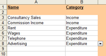
Column I uses VLOOKUP to return the category column for the categories list above.
P – Present the results

If you enjoyed this post, go to the top of the blog, where you can subscribe for regular updates and get your free report “The 5 Excel features that you NEED to know”.