

From the Not Just Numbers blog:
In my last post I described how to use both VLOOKUP and HLOOKUP to lookup and return data from lists or tables. Whenever I mention these functions in forums, etc. I usually get someone reminding me of how inefficient they are in terms of resource and how I should be using INDEX and MATCH.
I believe both approaches have their place – and use both where appropriate.
In a world of high speed processors and massive amounts of RAM (even on entry-level PCs), the resource issue t
On the other hand, INDEX and MATCH are incredibly powerful, more flexible and are less resource iends to only become relevant for those handling significant volumes of data. Meanwhile it is usually easier for most users to understand and use VLOOKUP and HLOOKUP.
ntensive for high volumes of data.
Horses for courses!
So for those of you who do deal with large volumes of data, or who are looking for greater flexibility than VLOOKUP and HLOOKUP can provide, here is how to do lookups using INDEX and MATCH.
First of all, let’s introduce the two functions:
INDEX is a function for returning a cell or range from within an array. At its simplest level this is done by referring to the cell by its row and column number (INDEX can do quite a bit more than this and also has another form which allows you to look at multiple ranges, however we only need to use its simple form here – I may do a post on some of its more advanced features at a later date). The simple form of INDEX is as follows:
=INDEX(range,row,column)
Column can be omitted and, if so, it is assumed to be 1 – unless range is just a single column in which case Excel will assume that the omitted argument is the row.
So for example:
=INDEX(A1:D5,2,3) returns the value in C2
MATCH finds the position of a value in a single row or column range. Its syntax is:
=MATCH(lookup value,range,match type)
match type is optional and has the following three possible values:
1 (or omitted) – finds the position of the largest value that is less than or equal to lookup value and requires the range to be in ascending order (this works the same way as using TRUE for the 4th argument in a VLOOKUP).
-1 – finds the position of the smallest value that is greater than or equal to lookup value and requires the range to be in descending order.
0 – finds the position of the first value that is exactly equal to lookup value (this works the same way as using FALSE for the 4th argument of VLOOKUP). In this case, the range can be in any order.
So if the range A1:A10, contains the values 5,6,3,8,12,4,9,34,23,54, then
=MATCH(4,A1:A10,0) returns 6, i.e the lookup value (4) appears 6th in the list.
Hopefully you are now starting to see how both these functions can combine to replicate a VLOOKUP (or HLOOKUP). We simply replace the row or column argument in the INDEX function with a MATCH function.
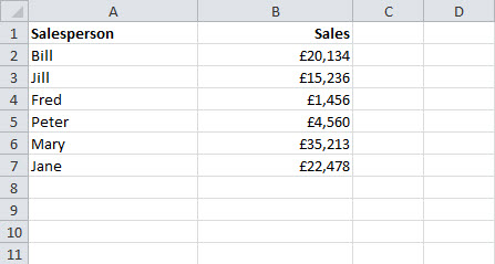
So for example in the following range:
If you enjoyed this post, go to the top of the blog, where you can subscribe for regular updates and get your free report “The 5 Excel features that you NEED to know”.