

From the Not Just Numbers blog:
This week you’ve got a break from me with a very useful guest post from Alan Murray of Computergaga.
Before we get into that though, just a quick reminder that the early bird discount on Mynda Treacy’s excellent Excel Dashboards course expires on Thursday, so if you don’t want to miss out, click over there now.
OK, on with Alan’s tips for when you don’t just want the average AVERAGE!
Calculating Median and Mode in Excel
When calculating averages in Excel, this normally involves using the AVERAGE function. The AVERAGE function in Excel calculates the mean of a set of numbers.
There are two other types of averages known as median and mode. Let’s take a look at calculating median and mode in Excel.

Calculating the Median
The median is the middle number in a sorted list of numbers. If you were to calculate the median with a pen and paper you would have to;
- Write down the list of numbers in numerical order.
- If there were an odd number of results, then the median would be the middle number.
- If there were an even number of results, then the median would be the mean of the two central numbers.
Fortunately Excel can handle all of this for us with the MEDIAN function. The following formula can be written to calculate the median from the list of exam scores.
=MEDIAN(B4:B13)
The list of exam scores is not sorted in numerical order, but that is no problem for Excel. The median has been found by finding the mean of 55 and 65 because there are 10 scores which is an even number of results.
39, 48, 51, 52, 55, 65, 75, 77, 77,90
(55 + 65) / 2 = 60
Finding the Mode
The mode, or modal number, is the number that occurs most frequently in a list. There can be more than one mode.
In Excel, the MODE function can be used on a list to return the number that occurs most often. In this example the formula would look like below.
=MODE(B4:B13)
The mode in this example can easily be seen to be 77 as it is the only one to appear more than once. If there is more than one modal number, this formula will only return the first one.
Returning Multiple Modes
To return multiple modes the MODE.MULT function can be used. This function was released with Excel 2010 so is not available on versions previous to that.
This function is an array function, so to run the function you should press Ctrl + Shift + Enter instead of only Enter. It will also appear in the Formula Bar wrapped within curly braces.
You will need to select a range of cells to apply the function to, or copy the formula and run it again.
In the example below there are 3 modal values. The following MODE.MULT function has been used in cells D5:D7 to return the results.
{=MODE.MULT(B4:B18)}

When there are no more modal values the function will return the #N/A error.
Watch the Video
Create a Frequency Distribution Table
Results are often broken down into groups, or classes. This
frequency distribution table gives us a good view of the spread of our data and
also identifies the class with the most occurrences, known as the modal class.
frequency distribution table gives us a good view of the spread of our data and
also identifies the class with the most occurrences, known as the modal class.
The table below shows the grades of 34 pupils in range
C4:C37.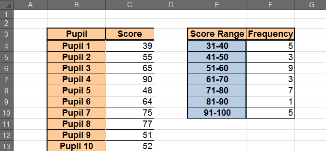
C4:C37.

The COUNTIFS function has been used to calculate these
frequencies. The formula below was entered into cell F4 and then copied to the
other cells of the table, with the criteria altered to match the class.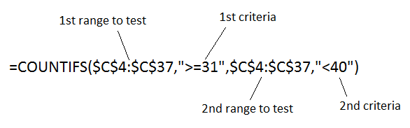
frequencies. The formula below was entered into cell F4 and then copied to the
other cells of the table, with the criteria altered to match the class.

The formula counts the number of scores that are greater
than or equals to 31, but less than 40. This is then repeated for each class.
than or equals to 31, but less than 40. This is then repeated for each class.
The COUNTIFS function was released with Excel 2007. If you
are using a version previous to this, the SUMPRODUCT
function could be used to count based on multiple conditions.
are using a version previous to this, the SUMPRODUCT
function could be used to count based on multiple conditions.
.
 About the author:
Alan Murray is an IT Trainer and the founder of Computergaga. Author of the
popular Computergaga Blog providing the latest Excel, Word, PowerPoint and Project tips and techniques.

If you enjoyed this post, go to the top of the blog, where you can subscribe for regular updates and get two freebies “The 5 Excel features that you NEED to know” and “30 Chants for Better Charts”.