From the Not Just Numbers blog:

Colour-coding can make it much easier for humans to read a spreadsheet, as our eyes and brains are wired up to treat differences in colour as important. For example, you may colour rows as red, amber or green based upon a status level – possibly, in a stock list, how close an item is to being out of stock.

If you do this, do you do it manually?

Many users know about Conditional Formatting, but do not know how to format whole rows in this way. I, for one, used it for years without knowing how to do this – but it’s really simple when you know how.

It involves using Conditional Formatting’s formula feature with Excel’s ability to fix references using the dollar sign.

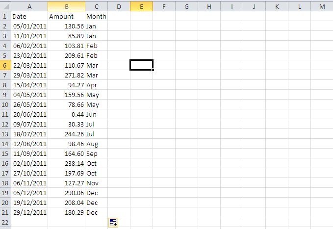
Let us take a very simple example of stock, where we wish to show lines with less than five items as red, less than ten items as amber and ten items or over as green.

Assume we have a heading row so the stock data starts at row 2, and the stock level is the last column of the data and is held in column H.

Highlight cells B2 to H1000, or down to whatever row more than covers the number of stock items you might have. Select Conditional Formatting (from the Home ribbon on Excel 2007/2010, or from the Fomat menu on Excel 2003) and select “Use a formula to determine which cells to format” (in 2007/2010) or “Formula is” (in 2003).

2003 and 2007/10 work slightly different in this respect, as 2003 allows you to add up to 3 conditions using the Add button and 2007/10 allows many rules to be added and managed.

The following formulae should be entered as the three conditions in Excel 2003, or as 3 separate rules in 2007/2010. In each case you will determine the format to be used if this condition is true using the Format button next to where you enter the formula. This works very similar to the normal dialogue box you get when formatting cells.

For the red:

Formula         =$H2<5
Format          Fill Red

For the green:

Formula         =$H2>=10
Format          Fill Green

For the amber:

Formula         =AND($H2>=5,$H2<10)
Format          Fill Orange

(read more on the AND function here, under combining conditions)

The most important thing to note here is the use of the dollar sign. What we are doing here is fixing the column (H), but leaving the row flexible, so that all cells in the highlighted range, look along their own row to column H to apply the criteria. Also note that you should enter the formula as if you were entering it for the first row of the range – this is why we have entered H2 as row 2 is the top row that we have highlighted.

One other thing to note is that the formula is always preceded by an equals sign, even if it has an equals sign in the criteria. So, if we had wanted to format red when H2 was equal to 5, we would have, rather oddly, entered =$H2=5.

This technique has many applications, and is really simple when you get the hang of it.

If you enjoyed this post, go to the top left corner of the blog, where you can subscribe for regular updates and get your free report “The 5 Excel features that you NEED to know”.

From the Not Just Numbers blog:

I see many time-saving tips for Excel users that speed up the time it takes to prepare a spreadsheet, such as keyboard shortcuts, text-to-columns, etc.

Where these are all very useful, I sometimes feel that an important truth is often overlooked.

A spreadsheet gets built once, but is used hundreds of times!

It is always worth having this at the back of your mind (or stuck on the wall above your desk!) when you are building a spreadsheet.

Anything that can be done when setting up the spreadsheet to speed up the experiencefor the user (even if that’s you) will pay for itself many times over.

This understanding can often be the difference between an amateur spreadsheet and a professionally produced one. They both do the job, but the good spreadsheet will let you do it in half the time, saving far more than the cost of doing it properly in the first place.

There are many ways in which a good spreadsheet does save the user time, such asdrop-down lists, logical data layout and conditional formatting, but the key is to know it’s important. If the user is having to copy and paste, change formatting or type something more than once, these are good indicators that the spreadsheet could have been better designed.

If this is the case, it is costing you every month, week or day (depending how often the spreadsheet is used) and it needn’t be the case. Take another look at it and see where it can be improved – or get it rewritten by a professional. Either way, you will be amazed at the time savings that are possible.

If you enjoyed this post, go to the top left corner of the blog, where you can subscribe for regular updates and get your free report “The 5 Excel features that you NEED to know”.

From the Not Just Numbers blog:

I come across many small businesses who use Excel (or Word) to produce an invoice template that they can email or print and post to their customers.

Usually the sale detail is entered on the face of the template and this is saved as a separate file for each invoice. The problem here is that to be able to report on this information for accounting purposes, or sales analysis, the information needs to be recorded somewhere else in one file (either another spreadsheet, or an accounting software package).

What is really needed is to be able to enter the sale details once and for this to be used to populate both the invoice template and the sales reports.

If an accounting package is being used, the best answer would usually be to use an invoicing module in the accounting software and ditch the external template, however if this is not an option, or an accounting system isn’t used, then we need the invoice template and the sales history to be linked.

Here is my approach to this problem, in the simple scenario where each invoice has one line of detail. If more lines are required a variation of this approach can be used, but this is a little too complicated to go into in this blog post.

General Approach
This approach involves three main worksheets within the one spreadsheet, Customer Data, Sales Data (what accountants often call a Sales Day Book) and the Invoice Template.

Customer Data
This worksheet, as the name suggests, is where all of the customer data is held. The sheet should follow the rules for laying out data that I outlined in an earlier post (How to lay out data in Excel). It should have column headings for name, address 1, address 2, etc. and one row for each customer, new customers are just added to the bottom of the list as needed.

The first column should be a unique identifier for that customer, it may be possible to use the name for this but you would need to add a new customer on a change of name rather than editing the existing one. Often better is to use the approach used by most accounting systems and allocate each customer a unique Account Code. I often use Conditional Formatting on this column to identify any duplicates.

The spreadsheet will use this sheet to provide the customer address details for the invoice.

Sales Data (or Sales Day Book)
This sheet should again follow the rules mentioned above. Here the business will record all sales, one line per sale. Headings should include (at least) Invoice No (in the first column), Date, Amount, Customer Account Code (the unique identifier mentioned in Customer Data above) and Description. Depending on needs the amount may be a calculated column, multiplying entries in columns for price and quantity. The business may also need a column for VAT or any other sales tax. The Customer Account Code column should use Data Validation to restrict entries to those codes in the first column of the Customer Data sheet.

The VLOOKUP function can then be used to pull in the customer name and address details in columns to the right of the entered data, using the customer account code to look that information up from the Customer sheet.


Invoice Template
If the business is already using an Excel template then this can be used as the basis of this sheet, otherwise some work will need to be done to produce a satisfactory layout for the invoice.

Ultimately there should only be one editable cell on these sheet – the Invoice Number which should be a dropdown based on the Invoice Number column of the Sales Data sheet.

VLOOKUP is then used on the rest of the invoice to pull the Customer Name and Address, Date, Description, Amount, etc. into the appropriate cells from the Sales Data sheet, based upon the Invoice Number selected.

I would recommend that to email the invoice to a customer, that it is printed to pdf first. This not only gets round the problem that all of your other sales data is in the same spreadsheet, but looks far more professional than sending a spreadsheet to the customer.

Reporting
As the sales data is all correctly laid out and, depending on the size of the business, at least a year’s worth of sales can be stored in the one spreadsheet (usually many more) then Pivot Tables can be used to report on these sales in any way that is required.

Just don’t forget to make sure you take regular backups and there is no need to record your sales anywhere else.

From the Not Just Numbers blog:

In my previous post, I stated that one of the major problems with how most Excel users lay out their data, is using a column for each category.

In the feedback I have had from that post, it was felt that this point needed further explanation and/or an example, so I thought I would provide both here.

First of all, here is the point as it appeared in the original post (it was point number 3):

Don’t group data by putting it in different columns (THIS IS THE ONE THAT ALMOST EVERYONE GETS WRONG)

1. • Don’t split out financial or numerical data into separate columns to categorise the data into months, expense categories, customers, agents, etc.
   • Do have one column for the financial or numerical data and create a column for month, expense category, customer or agent, to categorise each row;
   • You can use data validation drop-down lists to select the appropriate category for each row;
   • This one is counter-intuitive because in any report, you will almost certainly will want a column (or row) for each of these categories – but if you do this in the data you will massively restrict what you can do with it.

From the Not Just Numbers blog:

I’d really like to know what everyone thinks about this question – because I am not sure myself.

I have always fiddled with Excel until I got it to do what I wanted. For me, personally, it has worked out very well as I turned the skills I developed as a result into a successful business! But was it good for my employers at the time?

Granted, they got some good spreadsheet solutions in the end, but would it have been more effective to bring someone in who already knew how to do it, rather than use my time to get there by trial and error!

I’m sure I’m not alone as someone who likes to make sure they find a way, but it can be all too easy to spend far more time than could be justified in financial terms. Once the problem has been solved, the skills are there for next time, but is it the most efficient approach?

There are a few alternatives to fiddling with it until you get there using Google and Excel’s help facility, they all have a financial cost but can considerably reduce the time spent:

1. Excel training – this can obviously be useful but is often too generic to then apply to your real problems when you get back to the office. I have found a one-to-one approach is often more effective, working with the client’s own spreadsheets and problems. Another approach is to have training tailored to your business or industry (the service I offer to Accountants in Practice at Excellent Accountancy works along these lines)
2. Subscribe to a service where you have someone to ask – my Excel Advice by Email subscribers get this kind of service by email for just £75 per year
3. Get someone else to do it – I have my own service for this at needaspreadsheet.com

If you enjoyed this post, go to the top left corner of the blog, where you can subscribe for regular updates and your free report. If you wish to help me to provide future posts like this, please consider donating using the button in the right hand column.