From the Not Just Numbers blog:

Just a short post this week to tell you about a very handy little tool I found online.

If you develop as many spreadsheets as me, you will come across many situations where you need to enter some sample data into a spreadsheet to test it.

This can be pretty easy if it is numbers (you can use an excel function such as RANDBETWEEN, for example), but if you need a list of names, this can be a bit more tedious.

Aside: I’ve just realised that I don’t have an earlier post on random number functions to link to in the above pararagraph, so expect to see that in the next few weeks!

For names, I normally start making them up, but this gets harder than you think once you have exhausted Fred Bloggs, John Smith, etc! It’s also not the best use of my time!

I had a spreadsheet last week where I had to test it with the names of around 50 employees, which I had to make up. I thought a quick Google might be a better idea – and I came across a simple, yet ideal, on-line tool.

The perfectly titled listofrandomnames.com fitted the bill perfectly.

Within a few seconds I had 50 names to paste into my spreadsheet. I have to say that they weren’t necessarily everyday names, but that just made them a bit interesting. Who wouldn’t be impressed by a moniker as splendid as Sheridan Wolfenbarger?

There are a few quick choices to make:

• 5, 10, 20, 30 or 50 names?
• Male, Female or Both?
• First Names Only or Full Names?
• And even whether you require them to be alliterative!

If you enjoyed this post, go to the top of the blog, where you can subscribe for regular updates and get two freebies “The 5 Excel features that you NEED to know” and “30 Chants for Better Charts”.

From the Not Just Numbers blog:

Do you ever have those situations where you need to make an amendment to the text in every cell in a range?

I know it is an issue I come across regularly. I may need to prefix all nominal ledger codes with a department reference, say, or maybe add “/1” to all existing codes in a list, so that we can add new variations later of /2, /3, etc.

We could obviously rattle down the list, hitting F2 and pasting the additional text at the start or end of each cell. However, we can be a little cleverer than that.

Say we have the second situation described above and want to add “/1″ to every cell in the list. We can do this as follows.

If the list starts in cell A1, we could put the following formula in cell B1:

=A1&”/1”

This earlier post explains how to use “&” to join text together, as well as some other useful methods for manipulating text.

If we copy our formula down the whole list, column B will show the new text. We can then copy column B and paste it into column A. We will, however, need to do this using Paste Special, As Values. The easiest way to do this is to copy as normal but when pasting, right-click cell A1 and click the clipboard with “123” on it.

This will paste the results of the formula in column B (as opposed to the formula itself) as text into column A (replacing the original text). We can then delete column B (which will now be showing “/1″ twice in each row as it is being added to the new text in column A).

We can use the same technique with different versions of the formula to make any number of amendments to the text.

Say we want to add a department code before the code in column A and separate the two with a hyphen, we can enter the department codes in column B and enter the following formula (in column C):

=B1&”-“&A1

Use this technique with other text manipulation functions, from the post mentioned above, to make pretty much any change you need.

If you enjoyed this post, go to the top of the blog, where you can subscribe for regular updates and get two freebies “The 5 Excel features that you NEED to know” and “30 Chants for Better Charts”.

From the Not Just Numbers blog:

There are a number of situations, where it is useful to number each occurrence in a list.

We could place a flag in column B next to each occurrence using an IF statement, e.g.

=IF(A2=”North”,”Yes”,””)

Copying this down would place a Yes in column B next to each occurrence of North in column A, but it would not distinguish between each occurrence – they would all say Yes.

Fortunately there is a simple tip that you can use to place a number in column B, so that the first occurrence would show 1, the second 2, etc.

The principle is the same, we just need to replace “Yes” with something a little cleverer.

What we actually want now is to add 1 each time to the highest number already showing.

We can use the MAX function to find this highest number.

If we are again entering the formula in cell B2:

=MAX($B$1:$B1)

will return the highest number in the rows above (i.e. in cell B1).

Notice, though, the dollar signs. I have fixed both row and column on the start of the range, but only fixed the column on the end of the range. So copying this down, the end of the range would move, always going down as far as the cell above.

We can then use this formula, and add one, in place of “Yes” in our original:

=IF(A2=”North”,MAX($B$1:$B1)+1,””)

Whenever North appears in column A, this will find the maximum value in column B above this cell, and add 1 to it.

So, the first time North appears, there will be nothing above the row in column B, so 0+1=1. This will therefore return a 1 in column B.

Next time North appears, the maximum value in column B above this cell, will be 1 (returned against the first occurrence), so 1+1=2, etc.

We have all of our occurrences numbered in sequence now!

If you enjoyed this post, go to the top of the blog, where you can subscribe for regular updates and get two freebies “The 5 Excel features that you NEED to know” and “30 Chants for Better Charts”.

From the Not Just Numbers blog:

I received the following email from a reader and I thought it was a common problem that might make a good blog post.

Gill Carnell of www.secretsofsoftware.co.uk sent me the following email regarding her work with the First Monday Business Network in North Yorkshire:

“I have been running a Free business network event for just over a year now.

I have built up a spreadsheet of approx. 150 unique names/emails of those who have attended on one or more occasions. This main list increases by half a dozen or so each month.

I paste the main list to create an invitation list to promote an upcoming meeting via eventbrite.

After a few weeks I export the event registrations to a smaller spreadsheet. It contains mainly names from my main list plus new entries who have registered for the first time.

My mission is to then send a second invitation to those on the main list who have not registered (not on small spreadsheet).

Currently I’ve used various combinations of VLOOKP and MATCH functions to find entries on both lists. But then I have to filter or sort and then copy resulting values to create the new mailing list.

Question is whether there is an Excel Function or you can recommend a technique that allows two spreadsheets to be compared and if duplicates occur remove both entries, so I am not inviting people who have already registered? Sort of List One subtract List Two”

I think the simplest approach would be as follows:

Add two new blank sheets to the spreadsheet that contains the Main List, so that you can paste the Registrations list into one of them each time, and use the second for the mail merge.

Add a new column to the Main List to count entries on the second list.

Say that the Main List is on a tab called MainList and  the email addresses are held in column D, whereas the Registrations are held on a tab called Registrations, and that these email addresses are in column F.

The formula in this new column (for row 2) could then be:

=COUNTIF(Registrations!F:F,MainList!D2)

This can then be copied down to ensure that it covers the whole list.

This will count, how many times that email address appears on Registrations. We are only interested in the zeros (i.e. those that don’t appear on the Registrations List).

Switch on Autofilter for the main list (if it is not already switched on), and filter the Count column to only show zeros, then copy the list to the Mail Merge tab, which can be already set as the source for your mail merge.

Next time you do this, just delete the contents of the two spare tabs and paste the new registrations in. Your count column and Autofilter will already be set up and you mail merge will already be set up to point at the new list when you paste it into the mail merge tab.

I hope that helps Gill, and anyone else with a similar challenge.

If you enjoyed this post, go to the top of the blog, where you can subscribe for regular updates and get two freebies “The 5 Excel features that you NEED to know” and “30 Chants for Better Charts”.

From the Not Just Numbers blog:

Do you ever have a need to find the last row in a set of data – or the first gap?

I find that I use this tip quite regularly. It might be to help define a range to copy, or set a print area, or to identify where to enter the next row of data, or it might simply be that the last item in a list is highly relevant to the spreadsheet I’m developing.

Whatever the purpose, it is very handy to have a formula that will give me this information.

Say we want to know the first blank row in column A. We can use an array formula to return the row numbers of all the blank rows.

I will not go too much into array formulae here as that would be a significant blog post in itself, but there are three important things to know:

1. An array is a set of arguments or results, arranged into rows and columns, operations can be applied to the whole array
2. The result of an array formula will usually be an array itself and therefore will need another function to specify how it is to be shown as a single result (without this, the first result of the array will be displayed). Typical functions might be SUM or AVERAGE.
3. To enter an array formula, you need to press Ctrl+Shift+Enter, rather than just Enter

If you enjoyed this post, go to the top of the blog, where you can subscribe for regular updates and get two freebies “The 5 Excel features that you NEED to know” and “30 Chants for Better Charts”.

From the Not Just Numbers blog:

Named ranges can generate intense debate among Excel experts as everyone has their own views about how often they should be used – from those who argue that you should never directly address a cell in a formula (and should always give the cell (or range of cells) a range name, to those who only use them if they have to.

I would put myself somewhere in between the two extremes. There is certainly no denying that they can be a useful tool.

I don’t expect to resolve this debate here – I merely hope to introduce you to named ranges and how to use them.

Put simply, named ranges allow you to name a cell (or range of cells) so that this name can be used in a formula instead of the actual cell reference(s).

This provides the following advantages:

• It can be easier to see what’s going on in a formula if clear names are used;
• If a range needs to be extended or moved, the range can be edited once, rather than in every formula that refers to the range;
• Whereas inserting rows and columns, etc. will update both formulae referring directly to the moved cells and ranges, direct references from macros will not be updated. If the macro refers to a range name then this will not be a problem – as the range will have updated;
• Dynamic ranges – the definition of a range does not have to be a fixed reference and can be a formula. It can therefore be dependent on other variables in the spreadsheet .

 
If you enjoyed this post, go to the top of the blog, where you can subscribe for regular updates and get two freebies “The 5 Excel features that you NEED to know” and “30 Chants for Better Charts”.

Do you ever have those situations when you are trying different scenarios and constantly checking to see what effect your twiddling is having on your results?

Wouldn’t it be great if you could keep an eye on all of the cells you were interested in, without having to scroll all over the place?

Well, Excel has a nice simple tool to allow you to do exactly that.

The Watch Window tool is accessed from the Formulas ribbon, over to the right hand side of the ribbon.

When you click on the tool, it opens the Watch Window which hovers over the spreadsheet like any other toolbar.

Once the Watch Window is open you can add the cells that you want to keep your eye on by clicking Add Watch… and selecting the cells, either one by one or by selecting a whole range of cells. If you do this, all of the individual selected cells will be listed in the Watch Window. These cells can be on different worksheets and even in different workbooks.

For each cell, the Watch Window lists the Workbook, Worksheet, Name (if you have given the cell a name range), Cell reference, Value and Formula.

As you update the spreadsheet, the Watch Window will provide a live update of the effect on those cells. No more scrolling around!

Before I go, don’t forget that Mynda Treacy’s Excel Dashboards course is closing on Thursday, so get over there now if you don’t want to miss out.

If you enjoyed this post, go to the top of the blog, where you can subscribe for regular updates and get two freebies “The 5 Excel features that you NEED to know” and “30 Chants for Better Charts”.

From the Not Just Numbers blog:

Today’s post refers to a problem that started occurring in early December but I have had a number of clients raise the problem in recent days, as I think the Christmas break has probably meant the problem wasn’t noticed by many.

As a result, I thought it was probably still worth letting readers know about it in case they were experiencing it for the first time, or just had not managed to correct it yet.

The most common symptom of this problem is any ActiveX buttons in your spreadsheets ceasing to work. If this has happened to you and you haven’t yet found a solution, read on.

The problem stems from a Microsoft security update on 9th December and applies to the 2007, 2010 and 2013 versions of Office. If you have automatic updates switched on, you will have had this update.

The update has caused problems for ActiveX controls and the most visible problem is that existing ActiveX buttons, which you may have in your spreadsheet to run macros for example, just do nothing when you try to click on them. Note that Form Control buttons are unaffected.

Full instructions from Microsoft to deal with the problem are available here:

http://support.microsoft.com/kb/3025036/EN-US

In most cases, the following will work:

In File Explorer, search for all files ending in .exd, then delete these files (they are temporary files anyway and new ones will be created next time you use  the ActiveX controls).

At the Microsoft link above there is also a script that you can run to do this if you prefer.

Before you go, just a quick reminder that the 20% discount offer on Mynda Treacy’s Excel Dashboards course runs out on Thursday, so enrol now if you don’t want to miss out.

If you enjoyed this post, go to the top of the blog, where you can subscribe for regular updates and get two freebies “The 5 Excel features that you NEED to know” and “30 Chants for Better Charts”.

From the Not Just Numbers blog:

Before I get into this week’s post, I’d like to let you know that Mynda Treacy’s very popular Excel Dashboards course is once again open for enrolment. If you haven’t already taken this course, I’d highly recommend it, and you can get 20% off if you enrol by 22nd January. I’ll also throw in my Introduction to Excel PivotTables course free of charge, just enter FEECHAN in the Coupon Code field in the Cart or Checkout.

Anyway, on with this week’s post. Just a quick one this time.

In the comments of last week’s post, Bill Simpson of Texas mentioned a simple little tip that I hadn’t seen before. We’re all still learning!

I thought I’d share it with you all too.

If you want to enter the same thing into multiple cells, you can enter it into one and copy it into each of the other cells, however a quicker solution allows you to enter the same thing into all of those cells at once.

Just take the following steps:

• Highlight all of the relevant cells (you can use the mouse to highlight a range, or click on each of the individual cells while holding down the Ctrl key)
• While they are all highlighted, type what you want to
• Instead of hitting Enter, hit Ctrl + Enter, the information will appear in all of the selected cells.

If you enjoyed this post, go to the top of the blog, where you can subscribe for regular updates and get two freebies “The 5 Excel features that you NEED to know” and “30 Chants for Better Charts”.

From the Not Just Numbers blog:

Happy New Year everyone!

Welcome to the first post of 2015! I hope you’ve had a great break and are ready to explore more of what Excel has to offer in the New Year.

Many of you will know Bill Jelen from his many Excel books and/or his excellent (no pun intended) website, www.mrexcel.com. Well Bill is compiling a new book, MrExcel XL – 40 Greatest Excel Tricks and he sent me the following tweet over the Christmas break:

This was a tough challenge and the only way I could really think to address it was to look at the popularity (website traffic) of each of the tips that I post on here. This simplified the task hugely as there is one post that is consistently in the top three posts each month, even though it was written over three years ago. It is also something that I use in almost every formula I write!

My Greatest Excel Tip of All Time would be….

FANFARE….

“Learn how to use absolute references using $ and F4”

I have copied the information from my original post below, but if you like, you can still see the original, The dollar sign ($) in a formula – Fixing cell references, here.

Relative cell references
When you copy and paste an Excel formula from one cell to another, the cell references change, relative to the new position:

EXAMPLE:

If we have the very simple formula “=A1” in cell B1 it will change as follows when copied and pasted:

Pasted to B2, it becomes “=A2”

Pasted to C2, it becomes “=B2”

Pasted to A2, it returns an error!

In each case it is changing the reference to refer to the cell one to the left on the same row as the cell that the formula is in, i.e. the same relative position that A1 was to the original formula.

The reason an error is returned when it is pasted into column A, is because there are no columns to the left of column A.

This behaviour is very useful and is what allows a sum to be copied across or down the page and automatically refer to the new column or row that it finds itself in.

But in some situations, you want some or all of the references to remain fixed when they are copied elsewhere.

The dollar sign ($)
This is where the dollar sign is used.

EXAMPLE:

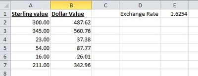
Take an example where you have a column of Sales values in Pounds Sterling in column A and a formula to convert these into US Dollars in column B. You could enter the actual exchange rate into the formula but it would be more sensible to refer to a cell where the exchange rate is held, so that it can be updated whenever it is needed.

The simple formula for cell B2, would be “=A2*E1”, however if you copy this down, then the formula in cell B3, would read “=A3*E2” as both references would move down a row as described above.

This is where the dollar sign ($) is used. The dollar sign allows you to fix either the row, the column or both on any cell reference, by preceding the column or row with the dollar sign. In our example if we replace the formula in cell B2 with “=A2*$E$1”, then both the “E” and the “1” will remain fixed when the formula is copied. i.e. in cell B3, the formula will read “=A3*$E$1”, still referring to the cell with the exchange rate in it.

In this example we have fixed both the row and the column, but in other situations, you may just want to fix one or the other, for example:

Above we have a spreadsheet calculating the times tables where we want to every cell in the white area to be the product of its row and column heading. This is easy using the dollar symbol. In cell B2, the formula without dollars would be “=A2*B1”, but for this formula to work when copied to each column, we need it to always look at column A for the first reference and to work for each row, we need to always look at row 1 for the second. Using the dollar sign to do this, it becomes “=$A2*B$1”. This can then be copied to every cell in the white area.

Quick Tip
You can speed up entering the dollar signs by using the function key F4 when editing the formula, if the cursor is on a cell reference in the formula, repeatedly hitting the F4 key, toggles between no dollar signs, both dollar signs, just the row and just the column.

If you enjoyed this post, go to the top of the blog, where you can subscribe for regular updates and get two freebies “The 5 Excel features that you NEED to know” and “30 Chants for Better Charts”.