From the Not Just Numbers blog:

In earlier posts you’ve heard me talking about the ICAEW’s Twenty Principles for Good Spreadsheet Practice.

This is a set of principles that, if you apply them, should significantly reduce the problem of spreadsheet risk, as well as make your spreadsheets far more robust and efficient.

The principles are now officially launched (to an audience of around 200 people at an event at Chartered Accountants’ Hall in London on June 17th) and free to download (I’ll give you the link at the end of this post).

The principles themselves are the work of the ICAEW IT Faculty Excel Community Advisory Committee, of which I am privileged to be a member.

The principles in brief are:

1. Determine what role spreadsheets play in your business, and plan your spreadsheet standards and processes accordingly.
2. Adopt a standard for your organisation and stick to it.
3. Ensure that everyone involved in the creation or use of spreadsheets has an appropriate level of know¬ledge and competence.
4. Work collaboratively, share ownership, peer review.
5. Before starting, satisfy yourself that a spreadsheet is the appropriate tool for the job.
6. Identify the audience. If a spreadsheet is intended to be understood and used by others, the design should facilitate this.
7. Include an ‘About’ or ‘Welcome’ sheet to document the spreadsheet.
8. Design for longevity.
9. Focus on the required outputs.
10. Separate and clearly identify inputs, workings and outputs.
11. Be consistent in structure.
12. Be consistent in the use of formulae.
13. Keep formulae short and simple.
14. Never embed in a formula anything that might change or need to be changed.
15. Perform a calculation once and then refer back to that calculation.
16. Avoid using advanced features where simpler features could achieve the same result.
17. Have a system of backup and version control, which should be applied consistently within an organisation.
18. Rigorously test the workbook.
19. Build in checks, controls and alerts from the outset and during the course of spreadsheet design.
20. Protect parts of the workbook that are not supposed to be changed by users.

If you enjoyed this post, go to the top of the blog, where you can subscribe for regular updates and get two freebies “The 5 Excel features that you NEED to know” and “30 Chants for Better Charts”.

From the Not Just Numbers blog:

First of all, it was great to see those of you that made it to last week’s launch event for the ICAEW’s Twenty Principles for Good Spreadsheet Practice. I hope to have a video of some of the highlights of the event to show you soon.

This week, I want to highlight an approach to copying and pasting that means you only bring across what you want, and don’t bring across any nasty surprises for later.

Have you ever opened a spreadsheet and been asked if you want to update links that you didn’t think were there?

…or ended up with a selection of different font sizes and formats in a range of data?

These are both signs of unwanted baggage dragged across during a copy and paste exercise, but can be easily avoided.

If you simply copy and paste, this brings across all formats and formulae from the source cells along with the contents, causing the two problems highlighted above.

Where the source cells have formulae that make reference to cells on other tabs of the source workbook, the pasted formulae will include external links back to the source spreadsheet. This causes the prompts about external links mentioned above. And, unless this is what was intended, a far greater problem is that the content of these cells will now update with changes to the source spreadsheet!

The multiple formats in a spreadsheet tend to come from pasting data from various sources with different formats.

Both can be easily avoided by some of the Paste Special options.

You can choose to bring over just the contents of the cells (no formats or formulae) by selecting to Paste Values , indicated by the clipboard showing the numbers 123. Note that the results of formuale are copied across as if they had been entered in the cell.

If you do want the formulae to be copied across, but not the formats, you can select Paste Formulas (the clipboard with fx on it).

You can also copy just the formats (leaving existing cell contents intact) by selecting Paste Formats (the clipboard with  a percentage sign and a paintbrush).

Finally, if you want to copy the cell contents and formats (but leave the formulae behind), you can select Paste Values and then Paste Formats.

There, you can now travel light when you’re copying and pasting!

If you enjoyed this post, go to the top of the blog, where you can subscribe for regular updates and get two freebies “The 5 Excel features that you NEED to know” and “30 Chants for Better Charts”.

From the Not Just Numbers blog:

Sometimes you have a spreadsheet that you want to look good and feel interactive, but might only have a few inputs.

A good example of this might be a loan illustration. You might want to experiment with different loan amounts, and terms for example.

You can of course just have an input cell for each of the variables (loan amount and term for example). But if you want to really jazz up the spreadsheet, what about interactive slider controls to enter the values, with the illustration responding to your movement of the sliders?

This is much easier than it sounds.

First of all, you will need to check that you have the Developer ribbon showing. If you do not have a ribbon called Developer, you can add it by clicking File, Options, Customize Ribbon and ticking Developer in the right hand column (Main Tabs).

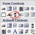
Now go to the Developer Ribbon and click Insert (it has a picture of a toolbox above it) and you will see the following options:

Select the option I have circled above and the cursor becomes a cross-hair for you to draw the rectangle that will become your slider.

Once you have drawn it, right-click on it and select Format Control.

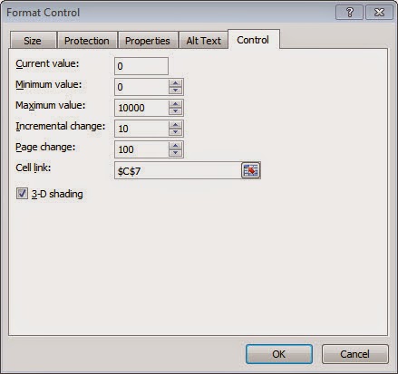
The screen above has all of the settings you need to make your slider work. The settings above could be for selection of Loan Amount in the example earlier. I will go through each in turn:

Current value – This is simply the value you want the slider to be set at before it is moved
Minimum value – The value when the slider is at the extreme left
Maximum value – The value when the slider is at the extreme right
Incremental change – How much you want the value to increase/decrease by when you click the arrow at either end
Page change – How much you want the value to increase/decrease by when you click the space between the selector and the arrow at either end
Cell link – The cell that you want the slider to link to. This will be the Loan Amount variable in the example described. In this case cell C7 will  show the value selected on the slider, and if you edit cell C7, the slider will move.

Have a play and see what you think.

If you enjoyed this post, go to the top of the blog, where you can subscribe for regular updates and get two freebies “The 5 Excel features that you NEED to know” and “30 Chants for Better Charts”.

From the Not Just Numbers blog:

Obviously, one of the most wonderful things about Excel is that you can refer to the contents of any cell by reference to its sheet, column and location and use those contents in a formula.

But what if you could store the row, column or sheet information in other cells that you could refer to to create the reference?

Well, you can, and, if you’ve lost me, I’ll tell you why you might want to!

The Excel function we can use here is INDIRECT.

This function asks Excel to treat the text between the brackets as a reference. To illustrate what I mean, let us assume that cell A1 contains the number 5 and cell A2 contains the text A1.

If in cell A3, we type the formula:

=A2

cell A3 will show the text A1 (i.e. the contents of cell A2)

If, however, we type the following into cell A3:

=INDIRECT(A2)

cell A3 will now show the number 5.

This is because we have told Excel not to return the contents of cell A2, but to treat those contents as a reference. So because A2 contains the text A1, the function now returns the contents of cell A1, i.e. the number 5!

This is most useful if you wish to build up a reference using text. For a refresher on manipulating text you might want to visit my earlier post:

Excel Tip: Manipulating text in Microsoft Excel

For example, we might want a formula to return the cell A1 from a particular tab, specified in another cell. So, say, cell B1 contains a drop-down of sheet names, our formula would be:

=INDIRECT(B1&”!A1″)

This takes the sheet name from cell B1 and adds the text !A1 on the end and then uses the INDIRECT function to treat the result as a reference, so if cell B1 contained Sheet2, then the reference would be Sheet2!A1.

This needs to be slightly more complicated if the sheet name could have spaces in it. When a sheet name has spaces, Excel requires it to be enclosed in single quotes, so Sheet2 is OK, but if you want a space, it must be ‘Sheet 2’. Excel will be happy with or without the single quotes when there is no space, so it is safer to include them. The formula would then be:

=INDIRECT(“‘”&B1&”‘!A1”)

There are many uses for INDIRECT, but I find manipulating the sheet name in this way to be one of the most useful.

If you enjoyed this post, go to the top of the blog, where you can subscribe for regular updates and get two freebies “The 5 Excel features that you NEED to know” and “30 Chants for Better Charts”.

From the Not Just Numbers blog:

Just a really simple tip this week, as the week started with a public holiday, both here and in the US. That means that you’re either lucky enough to have the week off and not interested in spreadsheets at all, or, like me, you’ve got four days to fit in a week’s work!

Have you ever inherited (I’m sure you wouldn’t have created one yourself) one of those Excel files with wild formatting all over it? 5 or 6 different fonts in as many different sizes and number formats, and twice as many colours?

Here’s a simple tip to strip it all away leaving you with the important stuff – i.e. the data in the cells.

First of all, highlight the range you want to clear (click in grey box in the top left corner of the screen, to the left of the A of the column headings and above the 1 of the row headings, if you want to select the whole sheet).

On the Home Ribbon, over to the right hand side of the screen (below AutoSum and Fill), there is a button called Clear (with a picture of an eraser next to it).

Click this and you will be presented with the following options:

• Clear All
• Clear Formats
• Clear Contents
• Clear Comments
• Clear Hyperlinks

If you enjoyed this post, go to the top of the blog, where you can subscribe for regular updates and get two freebies “The 5 Excel features that you NEED to know” and “30 Chants for Better Charts”.

From the Not Just Numbers blog:

Have you ever needed to sum the same cell across multiple sheets?

You might have 12 monthly sheets and an annual summary or 26 department sheets and a consolidation.

I don’t normally design spreadsheets that require this as it tends to go against my advice on how to structure your data.

I would generally advise one data input sheet that covers all months (or all departments) and a report that will present the information for any particular month (or department).

However, I see many spreadsheets that are structured like this and there are times when it is appropriate. In this post, I will show you a quick way to do it.

A reader asked me about this last week as she thought I had written about it in the past, and I had to look it up (as I said, I don’t normally have a need for it).

Before I looked it up, I would enter a formula such as:

=Worksheet1!A1+Worksheet2!A1+Worksheet3!A1+Worksheet4!A1+Worksheet5!A1

…to add cell A1 from 5 different worksheets.

This could get very tiresome, of you had, say, 100 worksheets!

The much more efficient way to do it is:

=SUM(‘Worksheet1:Worksheet5’!A1)

Note that it is the position of the worksheets that matters, not their name. The formula will sum all worksheets between Worksheet1 and Worksheet5 inclusive – left to right.

The reader, when I showed her this, remembered this useful tip from wherever she had read it. Use ‘bookend’ worksheets if the worksheets to add may change, e.g. have worksheets named First and Last, and place any sheets to be included in the sum in between them.

My thanks to the post that helped me to answer the question:

http://www.ozgrid.com/forum/showthread.php?t=73877

If you enjoyed this post, go to the top of the blog, where you can subscribe for regular updates and get two freebies “The 5 Excel features that you NEED to know” and “30 Chants for Better Charts”.

From the Not Just Numbers blog:

This week, I want to show you a neat little trick for doing something a little more visually interesting than just using brackets to distinguish between positive and negative variances.

In this post, I will show you how to automatically show a green thumbs up or a red thumbs down next to the variance (depending on whether it is good or bad).

Once you know how to do this you can replace these with arrows or some other symbols and make the colours whatever you want them to be.

OK. Say we have an actual figure in cell A1 and a comparison in cell B1. A1 might be this month’s sales, for example, and B1 might be budgeted sales, or last month’s sales. Either way, we want to make it obvious at a glance that A1 being higher than B1 is a good thing, and A1 being less than B1 is a bad thing.

A green thumbs up, or a red thumbs down, in cell C1, should make this pretty clear – so how do we do it?

First of all, where do we get the Thumbs Up and Thumbs Down symbols from?

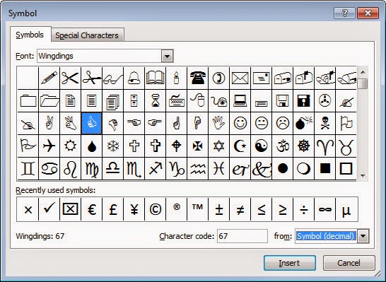
We can discover what symbols are available in different fonts by selecting Symbol from the Insert ribbon (this is on the far right of the standard Insert ribbon).

If we select the Wingdings font from the drop-down at the top, you can see there is a Thumbs Up symbol there. Click on it and note the number at the bottom left after the name of the font. In this case it says “Wingdings: 67”, so the number to note is 67. This is the character code of this symbol. Click on the Thumbs Down and you will see that this has a character code of 68.

OK, now cancel this screen, as we are going to insert these symbols in a different way – now we know what we want.

We can refer to any character by its character code using the CHAR function. So, if in any particular cell, we change the font to Wingdings (either by right-clicking and using the format cells dialog box, or by selecting the Wingdings font from the drop-down on the Home ribbon),

=CHAR(67)

will return the Thumbs Up symbol.

For our purposes, set the font in cell C1 to Wingdings and type the following formula into cell C1,

=IF(A1>=B1,CHAR(67),CHAR(68))

This formula will return the Thumbs Up character if A1 is greater than or equal to B1, and the Thumbs Down character, if it is not.

If you need a refresher on the IF function, take a look at this earlier post.

All we need to do now is change its colour. We can do this using Conditional Formatting.

First of all, change the font colour in cell C1 to green (again, either from th Home ribbon or Format Cells).

We then want this to change to red if C1 contains a Thumbs Down.

Click on cell C1 and from the Home ribbon, click Conditional Formatting, New Rule, Use a formula to determine which cells to format (this step is covered in more detail in this earlier post).

In the formula box, enter:

=C1=CHAR(68)

and click on the Format button to change the font colour to red.

That’s it. Change the values in A1 an B1 and you will see C1 change from a green Thumbs Up to a red Thumbs Down, depending on whether A1 is greater or less than B1!

As I said earlier in the post, you could use other symbols, such as up and down arrows and other colours, depending on your requirements. Have fun with it!

If you enjoyed this post, go to the top of the blog, where you can subscribe for regular updates and get two freebies “The 5 Excel features that you NEED to know” and “30 Chants for Better Charts”.